Special Scales

We have already seen how most slide rules, in addition to the basic C and D scales used for multiplication, have the A and B scales, useful for problems involving squares and square roots, the K scale for cubes and cube roots, the CI scale for reciprocals, and the L scale on which the common logarithms of numbers on the C or D scale can be read.

The Trigonometric Scales

Still more scales were very common on slide rules. Multiplying numbers by the sine, cosine, or tangent of an angle is something that one doesn't need to be a rocket scientist to have to do on occasion; even being a carpenter will suffice, and, therefore, trigonometric scales were, at least during the 20th Century, a standard feature even on most basic slide rules.

The S scale has marks that are labelled with angles in degrees; the location of each mark corresponds to the position on the C scale where the sine of that angle is found. Similarly, the T scale has marks that are labelled with angles in degrees, and the location of each mark corresponds to the position on the C scale where the tangent of that angle is found.

Thus, the S and T scales can be used for multiplying a number by the sine or tangent of an angle. And, of course, the cosine of 90 degrees minus an angle is the sine of that angle.

The tangent of an angle over 45 degrees is the reciprocal of the tangent of 90 degrees minus that angle. Thus, one uses the T scale to divide instead of multiply for such large angles. The number of degrees for such angles is thus noted in red on most slide rules, in the same way that the numbers on the CI scale usually are.

Usually, the center slide of even a simple slide rule had S and T scales. The simplest way to work with those scales is by flipping the center part over by taking it out of the side of the slide rule first, then flipping it over and putting it back in. But there were windows in the back of the slide rule that permitted using those scales without doing this, although one had to remember how to do that. The L scale was usually between the S and T scales on the back side of the center slide. On these slide rules, the S and T scales tended to be marked in degrees and minutes, and the S scale might work with the A and B scales while the T scale worked with the C and D scales.

The Log-Log Scales

The fancier slide rules also had a set of scales called "log log scales". What these scales let you do was raise numbers to arbitrary powers.

If the K scale, for example, shows the cube of numbers on the D scale by including three scales in the space of one, because adding the logarithm of a number to itself three times produces the logarithm of its cube, then one can cube a number by multiplying its logarithm by three.

And in that case, since a slide rule performs multiplication, a suitable scale should allow exponentiation.

This diagram illustrates a slide rule with a very small-scale log-log scale, matching the K scale. Usually, the log-log scale shown here would instead be broken into three pieces, called LL1, LL2, and LL3, matching the C scale.

The coarse resolution of the diagram above, and its small scale, shows the mark for 1.001 on the LL scale coinciding with the 1 on the K scale, but when the scale is made to correspond with the C scale, on a real 10 inch slide rule, a fourth piece, extending from 1.0001 to 1.001, called the LL0 scale, is worthwhile to provide, even if, for smaller numbers, the D scale will serve.

By shrinking the log-log scale down, I paired a scale with both it and the K scale in the diagram, to make the illustration simpler to understand.

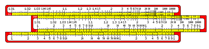
The J scale has been moved so that the 1 on that scale corresponds to the 3 on the K scale. Thus, every number on the J scale is multiplied by three on the K scale.

This displacement means that every number on the MM scale is cubed on the LL scale.

Thus, 1.01 is just past 1.03; 2 is under 8, 3 is under 27, 10 is under 1000.

Notice that the distance between numbers quickly shrinks. Thus, the tick marks between 100 and 1000 represent 150, 200, 250, 300, 350, 400, and 500.

While 10, 100, and 1000 stand in the same relation to each other on the LL scale as 1, 2, and 3 do on the K scale, note that 1.01, 1.02, and 1.03 also stand in approximately the same relationship to each other as 1, 2, and 3 do on the K scale.

This would let the K scale itself stand in for a lower extension of the LL scale, dealing with numbers like 1.001, 1.0001, and 1.00001. So the LL scale is aligned to facilitate that; 1.01 is placed near the index, instead of 10 being placed directly over 100 on the K scale.

This is done by placing a number on the log-log scale as follows: first, its natural logarithm is taken (just as the sine is taken first for the S scale), and then the common logarithm of that is taken to fit in with the other scales for multiplication. 1.01 to the 100th power is very nearly equal to e, and 1.001 to the 1000th power is even closer, and so on. So this is where we meet natural logarithms on a slide rule.

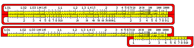
This diagram, placing the K scale directly against the LL scale, illustrates this more clearly, showing the two cases, the first where the correspondence shows with an alignment based on natural logarithms, and is an approximation approached in the limit, and the second where the correspondence is exact, and shows with an alignment based on common logarithms.

Incidentally, while most slide rules with log-log scales aligned them based on natural logarithms, one maker (Pickett) did use the common logarithm alignment. Also, some very old slide rules did have a log-log scale which was matched to the K scale for simplicity. Others, including the very first slide rule to have a log-log scale, aligned them with the A and B scales. On some such slide rules, the normal log-log scale was called the E scale, and the reciprocal log-log scale was called the F scale.

Many, but not all, slide rules with log-log scales also had reciprocal log-log scales (LL/3, LL/2, LL/1, LL/0 or LL03, LL02, LL01 and LL00) with numbers on them that were the reciprocals of those on the corresponding log-log scale, to allow numbers between 0 and 1 to be raised to powers as well without taking an extra step to calculate their reciprocals.

Most slide rules with both log-log and reciprocal log-log scales put the LL0 and LL/0 scales on the other side of the slide rule from the rest of the log-log scales; this was because all the ordinary scales were on the front, but there wasn't quite enough room for both log-log scales in full on the back. One of the few slide rules that avoided this was the Deci-Lon slide rule from Keufel and Esser, which is today one of the slide rules most sought after by collectors. It placed the four log-log scales on one side, and the four reciprocal log-log scales on the other.

The Faber-Castell Novo-Duplex, however, did even better, having all four segments of both log-log scales on one side. The Aristo 0969 StudioLog and the Aristo 0972 HyperLog were two other slide rules which had all four segments of both the normal and reverse log-log scales on one side and so did the Pickett Model 2, 3, and 4, N2, N3, N4, and 803, and the Flying Fish 1003.

The Faber-Castell Novo-Duplex (also sold as the Novo-Biplex in some countries) were also unique in having two sets of double-length scales for square roots which slid against each other, allowing higher accuracy in multiplication.

Incidentally, the log-log scale on the slide rule was first invented in 1815 by Dr. Peter M. Roget, a doctor of medicine, who is also the originator of Roget's Thesaurus. Although his invention was published in a scientific journal, it was largely forgotten, and the log-log scale was independently re-invented much later and on more than one occasion.

A few early slide rules that had only the LL2 and LL3 scales called them M and N.

Also, as the early practise on slide rules was just to allocate the letters A, B, C and D to the four main scales on the rule, whatever their type, the letters E and F were sometimes used for log-log scales, and sometimes for many other possible types of scale. The arrangement of scales was typically:

F A/B C/D E

and on one slide rule, the E scale might be an L scale, and the F scale might be a K scale, on another, the E scale might be the LL3 scale and the F scale might be the LL2 scale; on yet another, the E scale might combine the functions of the LL2 and LL3 scale, and operate with the A and B scales, while the F scale might similarly combine the functions of the LL02 and LL03 scales.

Slide Rule Scales: A Listing

Also, some slide rules had other special scales. A few of the more common of those, as well as the scales we have already discussed, are listed below:

• CF: This was a "folded" C scale, which was simply shifted so that the numbers marked on it were pi times the number on the C scale.
• CIF: This scale showed the reciprocals of the numbers on the CF scale.
• R1, R2 (or W1, W2): Instead of A and B scales, or in addition to them, some slide rules had a scale twice as long as the C scale, split into two halves to fit on the slide rule. This allowed calculations of square roots to be done with greater accuracy. (This was done on Versalog slide rules, for example.)
• T1, T2: Some slide rules included a second T scale so that tangents of angles over 45 degrees could be directly represented, instead of using additional (usually red) numbers indicating 90 degrees minus the angle on the T scale to allow the cotangent (the reciprocal of the tangent) of those angles to be found.
• ST or SRT: This is a folded C scale. Finding an angle on this scale in degrees allowed its equivalent in radians to be read off on the C scale. As sin(x) and tan(x) are very nearly x in radians for very small x, the primary use of this scale was to provide a backwards extension to the S and T scales.
• P: A number of slide rules, particularly those from Aristo, had this, the "Pythagorean" scale. A number x on this scale corresponded to sqrt( 1 - x^2 ) on the C scale (and vice versa, as this function is self-inverse) where the C scale is considered as containing the numbers from .1 to 1. This function was also one of the circle functions in APL along with the trigonometric functions, and could be used in calculating one side of a right triangle from the two others. This scale rapidly becomes very compressed near the right-hand side of the slide rule, so the fact that the function is self-inverse is helpful when using it for looking up the value instead of for multiplication in a subsequent step.
• Ln: A linear scale on a smaller scale than the L scale, this gave the natural logarithm of numbers from 1 to 10. Note that the log-log scales give natural logarithms in the same fashion that the S and T scales give sine and tangent, looking up the number on the scale which is the argument of the function, and finding the function's value on the C or D scale. This is the usual way in which scales associated with a function work, as this allows multiplying by that function of a number. But one doesn't usually multiply by a logarithm, and laying out the L and Ln scales in the reverse manner allows these functions to be looked up with constant percentage error in the argument and constant error in the result, which is a more reasonable distribution of error for logarithms.
• LL0, LL00: On a number of slide rules (the Post 1462, the Ricoh 150, the Dietzgen 1732 and 1735, and the Keuffel and Esser 4083-3) instead of these designations being applied to the first segment of the normal and inverse series of log-log scales, these two labels referred to the two parts of an inverse series of log-log scales that interoperated with the A and B scales; the LL0 scale corresponded to the conventional LL00 and LL01 scales, and the LL00 scale corresponded to the conventional LL02 and LL03 scales. On the Keuffel and Esser 4090-3, 4091-3, and 4092-3 slide rules, the LL0 scale, although it had 1/e at the index, was wrapped around so that it ran from the midpoint of the conventional LL01 scale at .97 to the midpoint of the conventional LL03 scale at .05. All these slide rules also had LL1, LL2, and LL3 scales of the normal type.
• BI: This scale was like the B scale, except that it ran backwards, bearing the same relation to the B scale as the CI scale did to the C scale. Thus, it allowed one to more quicly multiply by the reciprocal of a square root, by bringing the index of the slide against a number on the D scale instead of using the cursor.
• F or 2 pi: Electronic slide rules sometimes had a folded C scale which was folded at 1/(2*pi) instead of at pi. This was useful for calculations of the reactance of a capacitor (1/(2*pi*f*C)) or an inductor (2*pi*f*L).
• H or LC: This scale was like a BI scale, but was folded at 1/((2*pi)^2), which is approximately 0.02533. The resonant frequency of a tuned circuit with inductance L and capacitance C is 1/(2*pi*sqrt(L*C)), so one could divide either L or C on this scale by the other one on the B scale to read the resonant frequency on the D scale.
• Sd, Td, ISd, ITd: These scales show the ratio of the sine, tangent, inverse sine, and inverse tangent to their arguments (in degrees). These four scales have ranges that do not overlap, and thus they only occupy the same space as a single normal full-length scale. While these ratios are not often used directly in calculations, these scales can be used to provide sines and tangents with the same accuracy, and over the same range, as the complete set of four full-length scales S1, S2, T, and ST, and thus one maker of slide rules (P.I.C.) used these scales as a replacement for conventional trigonometric scales on some models of slide rule, despite the fact that this means that multiplying a quantity by the sine of an angle would take two steps instead of one.
• H and V or G: The H scale showed the square of the cosine of an angle (which equals one half of one plus the cosine of twice the angle), and was used in surveying for converting observations of stadia rods to distances. The V scale showed the product of the sine of the angle and the cosine of the angle (which equals half the sine of twice the angle), and was also used for this purpose. These scales were usually matched to the K scale of the slide rule, although there were exceptions. These two scales usually shared one line on the slide rule, and on some rules, the two together were called the G scale: specifically, the Dempster Rota-Rule model AA, and its descendant, the Pickett 110 ES.
• Th, Sh 1, Sh 2, Ch: Also, some slide rules had scales for some of the hyperbolic functions, hyperbolic tangent and hyperbolic sine. The hyperbolic sine occupied a split double-length scale. Hyperbolic cosine, although very rare, was provided on a few slide rules.
• H1, H2: The Aristo Hyperlog and the Flying Fish 1002 and 1003, which were also among the few slide rules to have a hyperbolic cosine scale, also had scales in which a number y on the C scale corresponded to sqrt( 1 + y^2 ) on this scale, and therefore a number x on this scale corresponded to sqrt( x^2 - 1 ) on the C scale, for yet another kind of scale that can be designated by the letter H on a slide rule. The H1 scale spanned the space corresponding to 0.1 to 1 on the C scale, and the H2 scale spanned the space corresponding to 1 to 10 on the C scale. These scales were called H2 and H3 on the Flying Fish 1002, which also called the P scale H'2, and they were called H0 and H1 on the Flying Fish 1003, which called the P scale H0 as well, but distinguished the scales only by slanting the label differently, and putting it in red, since like CI, the P scale runs from larger numbers to smaller from left to right: it is the nomenclature of the Aristo Hyperlog that I am taking as the standard.
• SR, TR1, TR2: Some slide rules had additional sine and tangent scales that took radian arguments. Although this would be particularly useful on a rule with hyperbolic trig functions as well, as the result would have been an unwieldy number of scales, other, less convenient, means of providing interoperability between hyperbolic and circular trig functions were used in slide rules like the Hemmi 153 (described below) and the Faber-Castell Mathema (which scaled the hyperbolic functions to be in degrees, except that instead of degrees at 360 to the circle, for both hyperbolic and circular trig functions, grads at 400 to the circle were used).
• M and X: On the Hemmi 257 chemical engineering slide rule, the M scale consisted of two decades of a scale that would have divided the rule into eight decades. The X scale was graduated with marks allowing the quantity x/(x+1) to be multiplied or divided, corresponding to x along the M scale; that is, if the position of a mark on the M scale is deemed to be log(x)/8, the position of a mark on the X scale is C + log(x/(x+1))/8, where C is a bit over 2.5 to allow a space between the scales. This allowed chemists to convert between mass ratios and molar ratios, and could be used to convert between volume and mass ratios or any other similar set of related ratios as well.
• Dynamo/Motor: This was a folded scale consisting of part of one decade of an A scale followed by one decade of an AI scale. The end index of both represented 100%, and was located over 7.46 on the A scale, as that represented a constant for converting kilowatts to horsepower. Since the efficiency of both a dynamo and a motor must be less than unity, and that of a dynamo is expressed in terms of kilowatts per horsepower, while that of a motor is expressed in terms of horsepower per kilowatt, this arrangement served to convert both to percents. When this scale was located on the body of the rule, the A scale represented kilowatts of electrical power, and the B scale represented mechanical horsepower.
• Volts: This scale served to indicate the voltage drop across a certain length of copper wire with a certain cross-sectional area, and again corresponded to the A and B scales. It could have different locations depending on whether English or metric units were used where the rule was to be used (the Dynamo/Motor scale, on the other hand, was fixed because it wasn't needed for metric units).
• U and V: On some other slide rules designed for electrical work, the V scale, used for calculating the voltage drop along a copper wire, was matched to the C and D scales, and the U scale, folded at pi/6, was also provided.

Slide rules with the scales for calculating reactance and resonant frequency often also had smaller versions of those scales on the back (repeated, and labelled with explicit magnitudes) to assist in locating the decimal point in such calculations.

One particular slide rule had a very large assortment of special scales. That was the Pickett N16-ES slide rule, designed by one Chan Street of Street Laboratory and Industries of El Segundo, California. This was a special-purpose slide rule designed for electronics calculations.

Even some of its ordinary scales were special; the S and T scales were actually SI and TI scales, giving the reciprocals of sines and tangents. This was done with the intent of facilitating polar to rectangular conversions. A Keufel and Esser slide rule, and some Hemmi slide rules, also had reversed sine and tangent scales, which were labelled as inverse scales in some cases.

The scales on the rule were organized into several groups.

• F, lambda, omega, tau: F represented the frequency of an alternating current, and was identical to the B scale, except that it explicitly ran from .1 to 1 to 10. Lambda represented wavelength; it ran from 3000 down to 30, and was the wavelength, in metres, of a wave whose frequency, in mHz, was given on the F scale, thus, it was a folded scale with the speed of light as the multiplying factor. The omega scale represents radians per second, and thus the number on that scale was 2*pi times the number on the F scale. The dimension on the tau scale was time, and its value was the reciprocal of that on the omega scale.
• C or L: This scale was used to determine either capacitative impedance, which is 1/(omega*C), or inductive impedance, which is omega*L. Since this scale was on the slider of the rule, along with the omega scale and its associated folded scales, it ran in the opposite direction to the omega scale to allow multiplication, and thus it was like a BI scale, except that, like the F scale, it ran from 10 to 1 to .1 explicitly.
• X sub L, X sub C: These represent inductive and capacitative reactance. (Impedance, usually noted by Z, is composed of both resistance and reactance, and X is the conventional symbol for reactance, the component of impedance due solely to the non-resistive quantities of inductance and capacitance, when it is noted as such.) The X sub L scale was a BI scale multiplied by 2*pi, and the X sub C scale was a B scale divided by 2*pi. Since the X sub L scale ran in the same direction as the C or L scale, one moved the desired number on the F, lambda, omega, or tau scale to the index point in the middle of the rule, and then read the impedance on the point on the X sub L or X sub C scale corresponding to the value on the C or L scale.
• C sub r, L sub r: This pair of scales was used to calculate the resonant frequency of an LC circuit. The formula involved is omega=sqrt(L*C). The C sub r scale was on the slider, and ran from 100 to 10 to 1 to .1 to .01. The L sub r scale, on the fixed part of the rule, ran in the opposite direction, so one placed the capacitance on the C sub r scale over the inductance on the L sub r scale, reading the square root of their product on the omega scale. Thus, the L sub r scale was folded by being divided by 4*(pi^2), compared to a scale running from 1 to 10,000, so the resonant frequency would normally appear on the left index of the rule.
• Cos theta, theta, (upper) db, D or Q: These scales represent, in different ways, the ratio between a resistance and a reactive impedance. The D or Q scale is identical to the A scale, except that it explicitly runs from .1 to 1 to 10. D is capacitative impedance divided by resistance, while Q is resistance divided by inductive impedance. The db scale was a linear scale, running from 60 to 20, so that a factor of 10 in amplitude represents 20 dB, corresponding to a hundredfold change of power. Theta (or alpha for the inductive case) being the phase angle, the D or Q scale showed the tangent of theta, from which theta and Cos theta derive as other functions of the ratio between reactance and resistance. Thus, theta equal to 45 degrees was found above the center index of 1 on the D or Q scale. The theta and cos theta scales were double scales, so that the tangent of theta could go from 10 down to .1 and then down to .001.
• (lower) db: On the lower part of the rule, a second db scale was present which was not linear. This scale indicated the losses caused by impedance mismatch, the degree to which power effectively applied to the resistance was less than that fed to the total complex impedance.

The Hemmi 269 slide rule was a slide rule which had stadia scales (that is, an H and V scale, simply labelled SIN COS and COS^2) which worked with the C and D scales, rather than the K scale. In addition, it had some extra scales:

• F: This scale was the successor to the A and K scales, giving the fourth power of numbers on the C and D scales: thus, numbers on this scale were positioned above their fourth root on the C and D scales.
• R: This was an additional B scale on the back of the rule; the R stood for 'radius'.
• TL: This scale worked with the R scale, and was a combined T1 and T2 scale; an angle on this scale was positioned above its tangent on the R scale.
• SL: This scale indicated the distance by which a rounded corner fell short of a pointed one; an angle theta on this scale would be positioned over (1/cos(theta)) - 1 on the R scale.
• CL: An angle on this scale corresponds to twice its equivalent in radians on the R scale; it is used for calculating the length along a rounded corner.
• M: An angle theta on this scale corresponds to 1 - cos(theta) on the R scale.

The Aristo Geodat had a two-part 1 - cos(theta) scale that operated with the C and D scales, in addition to a two-part stadia scale set that worked with the C and D scales like that of the Hemmi 269 and a scale used to enter the cotangent of half the angle in a calculation, for small angles running from one degree to one-tenth of a degree; this scale wrapped around, starting and ending in the middle of the rule. The same model number, 0958, was applied to versions of this rule using angles in degrees or grads (400 to the circle).

The Hemmi 266 slide rule, in addition to having scales for working out a*b by adding log(a) to log(b), thus finding 10^(log(a)+log(b)), had scales for finding sqrt(a^2+b^2) and 1/(1/a+1/b); the former were called the P and Q scales, the latter the R1 and R2 scales.

The Hemmi 153 slide rule had a unique complement of scales. In addition to a basic set of normal logarithmic scales, it had P and Q scales for finding sqrt(a^2+b^2) which were longer than those of the Hemmi 266, but in addition, it had a set of scales that worked in conjunction with those scales to give the values of both trignometric and hyperbolic functions.

It has a scale labelled with the Greek letter theta, giving angles in degrees. Corresponding positions on the R sub theta scale give its equivalent in radians, on the P and Q scales its sine, and on the T scale its tangent. As well, the G sub theta scale gave the Gudermannian of the value on the R sub theta scale, so that starting with a value on the G sub theta scale, its hyperbolic sine was in the corresponding position on the T scale, and its hyperbolic tangent in the corresponding position on the P and Q scales.

Slide rules for business use sometimes had a linear scale which was used for calculating the number of days between two dates. A similar scale could be used to make a perpetual calendar: the days of the week might be symbolized by a pattern of tick marks like this:

 ||||||||||||||
  |||||  |||||
  |||||  |||||
  | | |  | | |

with short ticks representing the weekend, and the longest ticks representing Monday, Wednesday, and Friday so that the alternating pattern allows recognizing any day of the week quickly. The scale of days of the week could be positioned against the scale showing the days of the year by bringing, further along the scale, a mark for the century opposite a mark for the year of the century.